The effective interest rate is the difference between those two views summed with the gap between actual and expected inflation. In this post, I use a simple IS/LM framework to derive time preferences over the last 55 years and calculate the effective interest rate. As demonstrated in Chart 1 below, effective interest rates calculated in such manner exhibit strong negative correlation to consumption growth.

Let's start with the problem. Macro-economic models assume positive time preferences which are stable over time. The problem is that the models do not fit historical data on consumption. In Noah Smith's own words:
Furthermore, experimentation has shown that simple re-framing of choices can lead to negative time preference. Here's another excerpt:Basically, it [Consumption Euler Equation] says that how much you decide to consume today vs. tomorrow is determined by the interest rate (which is how much you get paid to put off your consumption til tomorrow), the time preference rate (which is how impatient you are) and your expected marginal utility of consumption (which is your desire to consume in the first place).
This equation underlies every DSGE model you'll ever see, and drives much of modern macro's idea of how the economy works. So why is [Martin] Eichenbaum, one of the deans of modern macro, pooh-poohing it?
Simple: Because it doesn't fit the data. The thing is, we can measure people's consumption, and we can measure interest rates. If we make an assumption about people's preferences, we can just go see if the Euler Equation is right or not!
Experimental and field research has shown that individuals often exhibit time inconsistent preferences.Before jumping into the methodology behind the historical data set in Chart 1 above, let's start with some econ 101. Why do savers demand interest in order to extend credit, and why do borrowers willingly pay interest in order to receive credit? Setting credit risk and inflation expectations aside, savers and borrowers have to consider the marginal utility of consumption today and compare it to the utility of future consumption. If you expect your future wealth to double, spending $100 today will bring you a lot more marginal utility compared to spending $100 in that blissful future when all of your needs will be satisfied. Accordingly, a saver will demand interest to compensate for the loss of utility associated with delayed consumption. For the very same reason a borrower is willing to pay interest. By spending the borrowed money today, a borrower gains utility compared to the future utility he or she forgoes upon paying back the debt. Time preference is exactly the perceived utility difference between current and future consumption. And just like Noah Smith suggests, time preference is always framed in terms of expectations of our future wealth. As expectations change, so do our time preferences.
...
Now, here's the thing...it gets worse. [David] Eil, though a very careful and expert experimentalist, is not the only person to do experiments on time-discounting; it is a very common research topic. And I've heard whispers that a number of researchers have done experiments in which choices can be re-framed in order to obtain the dreaded negative time preferences, where people actually care more about the future than the present! Negative time preferences would cause most of our economic models to explode, and if these preferences can be created with simple re-framing, then it bodes ill for the entire project of trying to model individuals' choices over time.
Now, let's flip things around and suppose that people expect to be poorer in the future. If you expect your future wealth to decline by half, saving $100 today when you are relatively well-off and setting it aside for a rainy day will result in higher future marginal utility. Under such scenario, delayed consumption results in a gain for the saver and a loss to the borrower. This is the equivalent of a negative time preference (when you discount with a negative discount factor, future value is higher than present value). In order to induce the borrower to take on more credit, the interest rate has to be negative. And here comes the catch, savers can arbitrage negative rates by simply holding cash or bank deposits at 0%. This is the realm of the feared lower zero-bound, which is characterized by a glut of savings, a shortage of borrowing and depressed economic activity.
If total savings equaled total borrowing, the interest rate charged in financial markets would be equal to the time preference in the real economy. However, the fact that money can be held as an asset makes it possible for savings to exceed borrowing as in the case of the lower zero-bound. In addition, fractional banking can enable an excess of borrowing over savings. Banks can simply expand the money supply in order to meet excess loan demand. As a result interest rates and time preference do not have to match. In order to derive time preference, we have to consider a hypothetical monetary system where savings always equal borrowing (basically, for every saver there has to be a corresponding borrower who is not a bank). So the task of finding time preference over time is equivalent to finding the equilibrium rate of interest for each historical period.
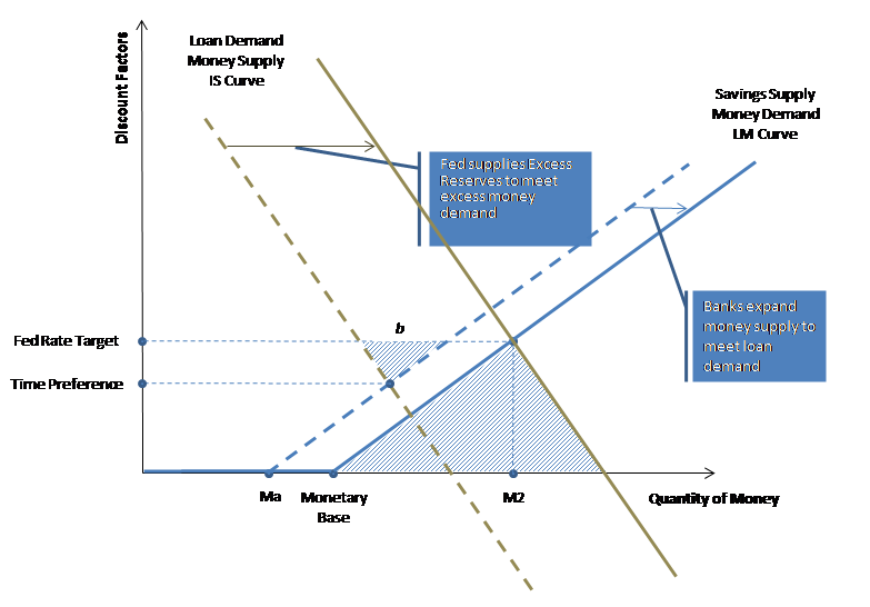
Next let's review Chart 2 below, which illustrates the IS/LM model used to derive the historical time preference rate.

The solid IS and LM curves represent the actually observed state at a specific point in time. The dotted curves represent the hypothetical scenario at which savings and borrowing equal without the distorting effects of money and the banking system. Suppose the Federal Reserve sets the interest rate target (Fed Rate Target) below the Time Preference rate. At that level, demand for loans exceeds the supply of savings, and banks expand the money supply to meet the excess loan demand as represented by the LM curve shift to the right. The Fed stands ready to accommodate such shift by supplying the necessary level of reserves as represented by the observed Monetary Base (MB). Please note that if the Fed did not supply such reserves, the interest rate will go above the Fed Rate Target. In a previous post on asset bubbles, I explain how to derive Ma, which is the level of asset money demanded by the public. Ma represents the hypothetical monetary base had it not been for the distorting influence of banking and the Fed. Please note that a traditional IS/LM model shows Output on the horizontal axis. In this modified model, output is represented by Mt (transaction money or the difference between M2 and Ma which directly correlates to GDP). Now that we have the Fed Rate Target (R), Asset Money (Ma), the Monetary Base (MB) and Money Supply (M2), we can derive both the hypothetical and actual LM Curves.
The next step is to derive the IS curves. We have one point on the solid IS curve, which is the intersection of the Fed Rate Target (R) and M2. I derive the slope of the IS curve by plotting historical money expansion (M2 less MB) against real interest rates as shown in the chart below.

Using the slopes as regressed above I can now derive the IS curves as well. The difference between the hypothetical IS curve and the actual is represented by Excess Reserves (E) provided by the Federal Reserve. Generally, sizable excess reserves exist when the Fed Rate Target is above the Time Preference which creates a shortage of money with the lower zero-bound being a perfect example. Chart 4 below illustrates the IS/LM model with significant Excess Reserves.
Side b of the smaller highlighted triangle can be calculated as follows: b = MB - Ma - E (Monetary Base less Asset Money Demand less Excess Reserves). A positive value for b means that the Fed Rate Target is below Time Preference as in Chart 2. A negative value for b means that the Fed Rate Target is above Time Preference as in Chart 4.
With this framework and monetary data provided by the St. Louis Fed, historical time preferences can be easily derived going as far back as the late 1950s. The effective interest rate (ER) as presented in Chart 1 is calculated as follows: Effective Interest Rate (ER) = Fed Rate Target (R) - Time Preference (T) + Inflation Adjustment (IA). For each period, the inflation adjustment stands for the difference between actual inflation over the prior 12 months and inflation expectations as measured by the actual inflation over the following 12 months. Basically, if inflation over the prior 12 months is let's say 4%, but expected inflation over the next 12 months is 3%, the public perceives 1% higher effective rate. The reason for this could be the public's perception that interest rates today reflect prior inflation experience but not their individual expectations for future inflation.
Charts 5, 6 and 7 below show the results of the historical analysis.


I think what is more interesting is the significant influence exerted by the inflation adjustment. The inflation adjustment is by far the bigger component of the effective rate. Again, the inflation adjustment is equal to the difference between future inflation and past inflation. That such measure should have a significant influence on consumption growth is interesting and curious and could be a leading indicator. Please note that the consumption growth in Chart 1 is calculated as the growth compared to the prior-year period. In the data set, I used the actual inflation over the following 12 months to approximate inflation expectations; however, surveys of inflation expectations could be used as a proxy to project consumption in current quarter. Anyway, I don't think I fully understand the meaning of this relationship, and it definitely warrants more study.
To conclude, it does seem intuitive that time preferences are always framed in terms of people's perceptions of their future wealth. Accordingly, as such expectations change, time preferences should change as well. Negative time preferences also make perfect sense. Saving for a rainy day is common folk wisdom. Starting from this simple intuition, I've attempted to lay out a framework for deriving time preferences in the real economy from widely-available historical data sets of monetary aggregates. The historical analysis seems to confirm the intuition.
No comments:
Post a Comment